模拟退火算法

背景介绍

SA(Simulate Anneal):是一种基于Mentcarlo迭代求解法的一种启发式随机搜索方法，基于物理中固体物质的退火过程与一般组合优化问题之间的相似性，通过模拟退火过程，用来在一个大的搜寻空间内找寻命题的最优解（或近似最优解）。

核心思想

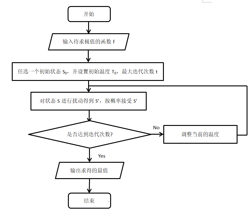
1. 任选一初始状态S₀作为当前解，设置初始温度T₀

2. 对该温度下的状态S₀产生一个扰动S’，并按概率接收
$$\Delta C=f(S’)-f(S)$$

$$P= \begin{cases} 1 & \Delta C \leq 0 \ e^{\frac {- \Delta C}{T} } & \Delta C > 0 \end{cases}$$

3. 按照某种方式降温T=T-ΔT，回到步骤2，直到满足某个终止条件

4. 此时达到的状态S即为该算法的最优解

算法流程

代码实战

代码中所用测试函数可以查看相关文档，测试函数(Test Function)

SA_ap.m

clear;clc;close all;
%自变量取值范围
range_x=[ones(1,1),-ones(1,1)]*500;
%维度
n=size(range_x,1);
%尝试解次数
num=10;
value=zeros(n,num);
delta_t=0.2;
tic;
for i=1:num
    %给x赋初值
    x=zeros(n,1);
    for k=1:n
        x(k)=(rand(1))*(range_x(k,2)-range_x(k,1))+range_x(k,1);
    end
    %初始温度t
    t=100;
    while t>1e-5
        x=SA_metripolis(range_x,t,x,n);
        %温度每次下降delta_t
        t=t-delta_t;
    end
    value(:,i)=x;
end
time=toc;
disp(['用时：',num2str(time),'秒'])
[mini,index]=min(f(value));
disp(['fmin=',num2str(mini)]);
for k=1:n
    disp(['x',num2str(k),'=',num2str(value(k,index))]);
end
if n==1
    hold on;
    plot(value(index),mini,'ro');
    plot_x=range_x(1):(range_x(2)-range_x(1))/1000:range_x(2);
    plot_y=f(plot_x);
    plot(plot_x,plot_y);
    text((range_x(1)+range_x(2))/2,max(plot_y)+0.1*(max(plot_y)-min(plot_y)),['用时：',num2str(time),'秒']);
    hold off;
end
if n==2
    %所求最小值的函数
    func=@(x1,x2)x1.*sin(sqrt(abs(x1)))+x2.*sin(sqrt(abs(x2)));
    plot_x=range_x(1,1):(range_x(1,2)-range_x(1,1))/1000:range_x(1,2);
    plot_y=range_x(2,1):(range_x(2,2)-range_x(2,1))/1000:range_x(2,2);
    [plot_x,plot_y] =meshgrid(plot_x,plot_y);
    plot_z=func(plot_x,plot_y);
    surf(plot_x,plot_y,plot_z);
    xlabel('x1');
    ylabel('x2');
    zlabel('y');
    hold on;
    plot3(value(1,index),value(2,index),mini,'ko')
    text((range_x(1,1)+range_x(1,2))/2,(range_x(2,1)+range_x(2,2))/2,max(max(plot_z))+0.5*(max(max(plot_z))-min(min(plot_z))),['用时：',num2str(time),'秒']);
    hold off;
end

SA_metripolis.m

function x=SA_metripolis(range_x,t,x,n)
delta=1;
for i=1:100
    %产生一个随机扰动
    x_new=(rand(n,1)-0.5)*delta+x;
    %限制解的范围
    for j=1:n
        if x_new(j)<range_x(j,2)
            x_new(j)=range_x(j,2);
        end
        if x_new(j)>range_x(j,1)
            x_new(j)=range_x(j,1);
        end
    end
    dc=f(x_new)-f(x);
    if dc<0
        x=x_new;
        %如果扰动的结果比原来大，则有概率的保留
    else
        p=exp(-dc/t);
        if rand(1)<=p
            x=x_new;
        end
    end
end

f.m

function res=f(x)
func=@(x)(x).*sin(sqrt(abs(x)));
res=zeros(1,size(x,2));
for i=1:size(x,1)
    res=res+func(x(i,:));
end

实验结果

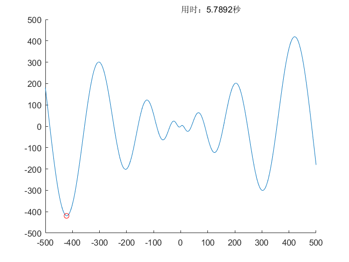
$$f(x)=x \cdot \sin(\sqrt{\lvert x \rvert}) \ , \ x \in [-500,500]$$

$$理论值：f(x)_{min}=f(-420.96874592006)=-418.982887272434$$

$$所求值：f(x)_{min}=f(-420.967823415805)=-418.982887164947$$

性能比较

优点：
- 计算过程简单
- 可用于求解复杂的非线性优化问题
- 相比梯度下降，增加了逃离局部最小的可能

缺点：

参数敏感
收敛速度慢
执行时间长
算法性能与初始值有关
可能落入其他的局部最小值