Scikit-Learn介绍
Scikit-Learn库自2007年发布以来,已经称为最受欢迎的机器学习库之一,基于广受欢迎的Numpy和Scipy库构建,能够提供用于机器学习的算法,数据预处理等功能。
Scikit-Learn应用
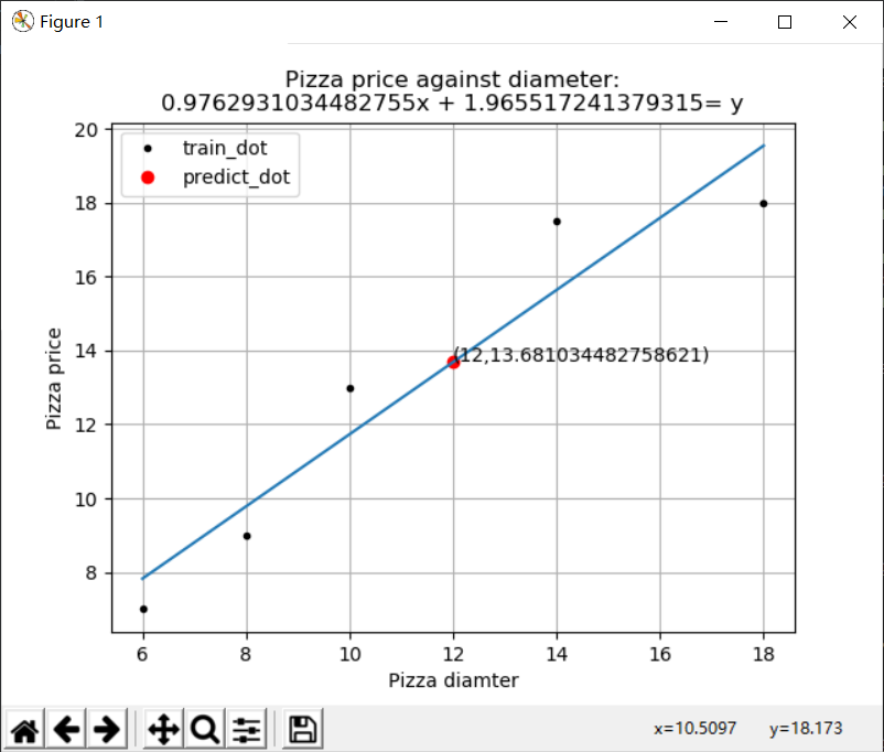
Scikit-Learn线性回归
1 | import numpy as np |
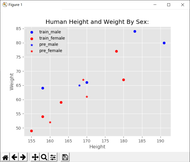
Scikit-LearnK近邻分类算法
1 | import numpy as np |
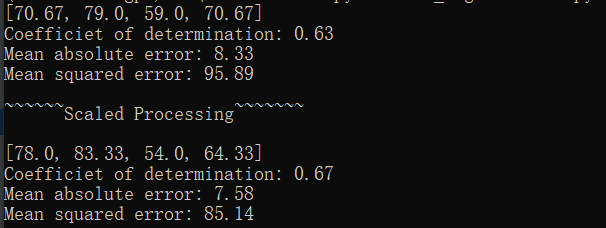
Scikit-LearnK近邻回归算法
1 | import numpy as np |
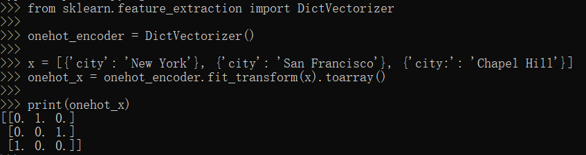
Scikit-Learn独热编码
1 | from sklearn.feature_extraction import DictVectorizer |
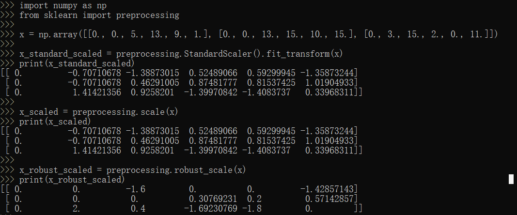
Scikit-Learn特征标准化
1 | import numpy as np |
Scikit-Learn多元线性回归
1 | from sklearn.linear_model import LinearRegression |
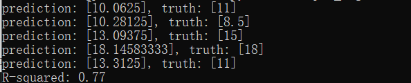
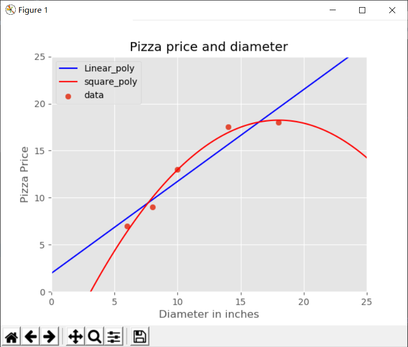
Scikit-Learn多项式回归
1 | import numpy as np |
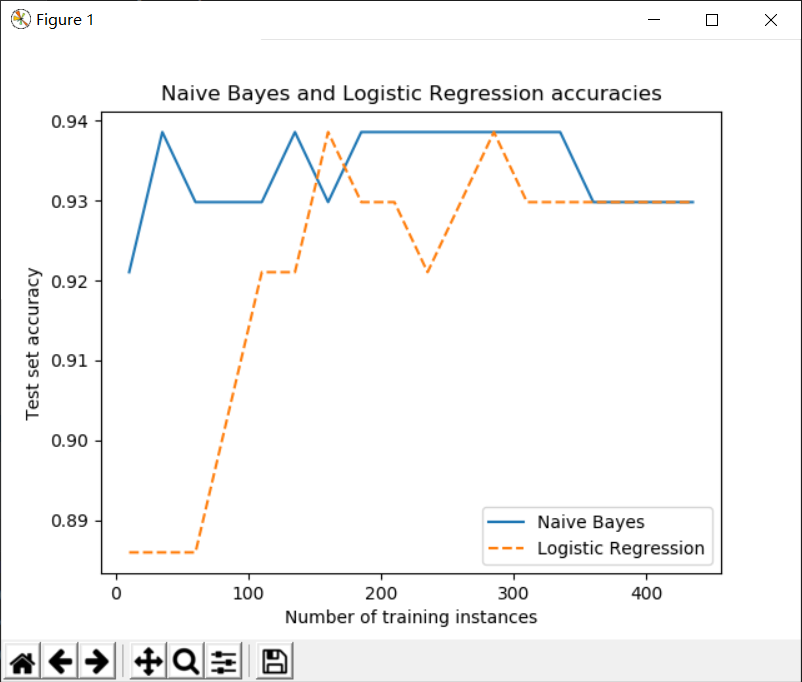
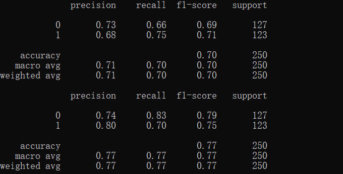
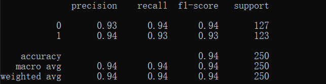
Scikit-Learn逻辑回归和朴素贝叶斯
1 | from sklearn.datasets import load_breast_cancer |
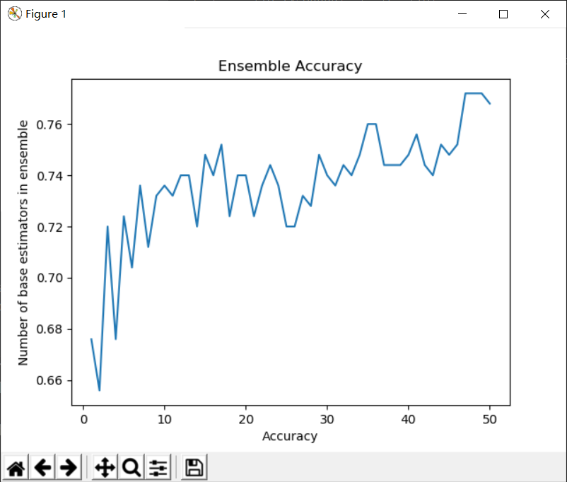
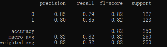
Scikit-Learn决策树和袋装集成学习
1 | from sklearn.tree import DecisionTreeClassifier |
Scikit-Learn推进集成学习
1 | from sklearn.ensemble import AdaBoostClassifier |
Scikit-Learn感知机
1 | from sklearn.datasets import make_classification |
Scikit-Learn支持向量机
1 | from sklearn.datasets import make_classification |
Scikit-Learn多层感知机
1 | from sklearn.datasets import load_digits |

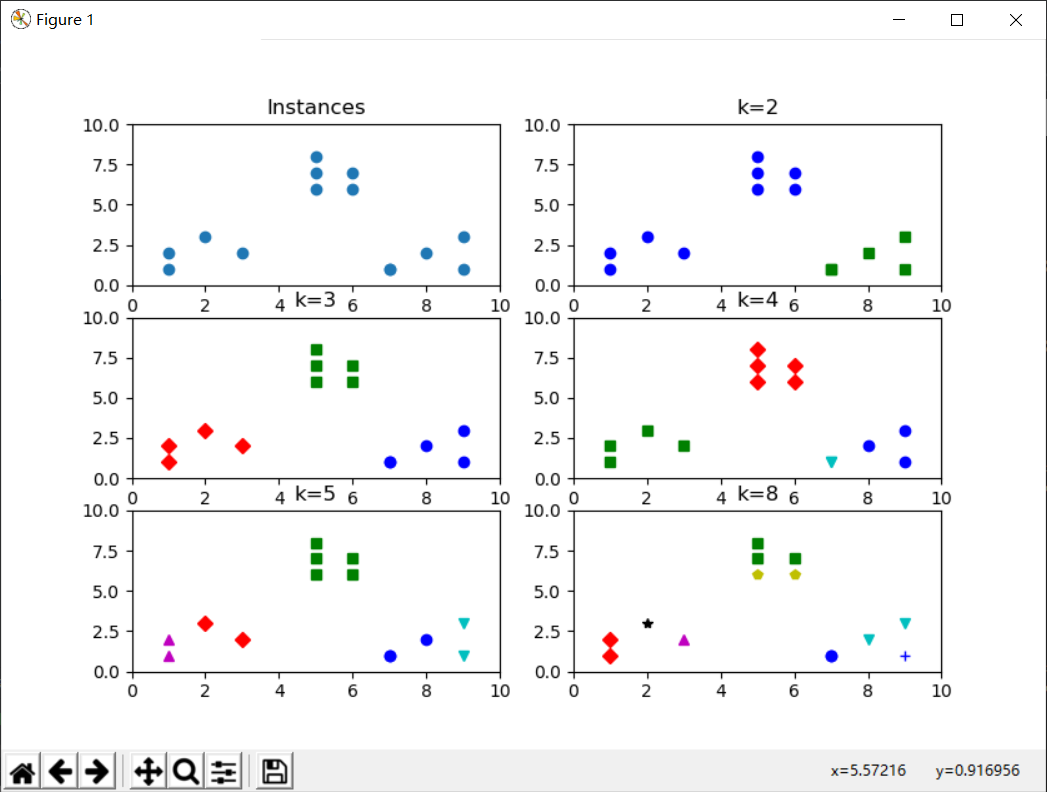
Scikit-LearnKmeans聚类
1 | import numpy as np |
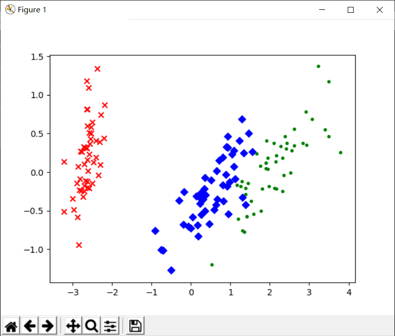
Scikit-LearnPCA降维
1 | import matplotlib.pyplot as plt |
Scikit-Learn小结
由于Scikit-Learn集成了许多常用的机器学习算法,如决策树,SVM,多层感知机,Kmeans等,可以让使用者节约大量的时间。而且其拥有很好的官方文档,让开发者,研究者可以方便的入门和使用。因此Scikit-Learn在机器学习领域受到广大使用者的喜爱。